Creating Fields
There are a few ways to get the benefits of using viscid.Field (coordinate aware ndarrays). The easiest is to use the readers built into Viscid (through viscid.load_file()). If there is no reader for your data format, you can wrap arrays in a number of ways…
Constructing a Field From Scratch
Viscid has viscid.empty(), viscid.full(), viscid.zeros(), viscid.ones(), viscid.empty_like(), viscid.full_like(), viscid.zeros_like(), viscid.ones_like() that work just like their numpy counterparts. Here are some examples how to use them,
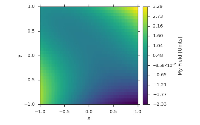
Scalar Field
import numpy as np
import viscid
from viscid.plot import vpyplot as vlt
import matplotlib.pyplot as plt


# Make some coordinate arrays. These happen to have uniform grid spacing.
# In most cases, Viscid will notice that and make a uniform coordinates.
# Interpolation / streamline calculation is faster on uniform fields than
# nonuniform (rectilinear) fields.
x = np.linspace(-1, 1, 64)
y = np.linspace(-1, 1, 32)

# create a new field
fld = viscid.empty([x, y], center='cell', name="MyField",
                   pretty_name="My Field [Units]")

# fill the field with data... shaped crds are a lightweight way
# to broadcast to the field's shape
X, Y = fld.get_crds(shaped=True)
fld[...] = X**2 + Y**3 + 2.0 * X * Y - 0.5 * X

plt.figure(figsize=(8, 5))
vlt.plot(fld)
vlt.auto_adjust_subplots()
plt.show()
(Source code, png)
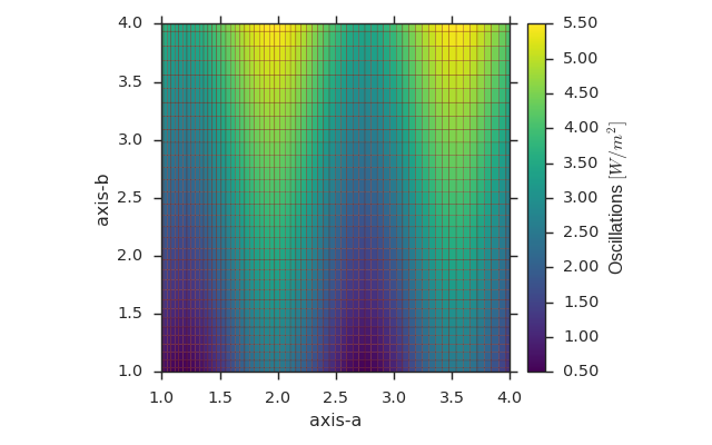
Scalar Field with Custom Coordinate Names
import numpy as np
import viscid
from viscid.plot import vpyplot as vlt
import matplotlib.pyplot as plt


# now the coordinates are rectilinear, and that's ok too
a = np.linspace(1.0, 2.0, 64)**2
b = np.linspace(1.0, 2.0, 32)**2

# create a new field, this time it's node centered
fld = viscid.empty([a, b], crd_names=('axis-a', 'axis-b'), center='node',
                   name="Oscillations", pretty_name="Oscillations $[W/m^2]$")

# fill the field with data... shaped crds are a lightweight way
# to broadcast to the field's shape
A, B = fld.get_crds(shaped=True)
fld[...] = np.sin(4 * A) + B + 0.5

plt.figure(figsize=(8, 5))
vlt.plot(fld, g='#7C1607')
vlt.auto_adjust_subplots()
plt.show()
(Source code, png)
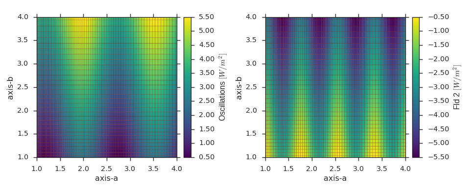
Scalar Field on the Same Grid as an Existing Field
import numpy as np
import viscid
from viscid.plot import vpyplot as vlt
import matplotlib.pyplot as plt


a = np.linspace(1.0, 2.0, 64)**2
b = np.linspace(1.0, 2.0, 32)**2

fld1 = viscid.empty([a, b], crd_names=('axis-a', 'axis-b'), center='node',
                    name="Fld1", pretty_name="Oscillations $[W/m^2]$")
A, B = fld1.get_crds(shaped=True)
fld1[...] = np.sin(4 * A) + B + 0.5

# create and fill a field like fld1
fld2 = viscid.full_like(fld1, np.nan, name='Fld2',
                        pretty_name="Fld 2 $[W/m^2]$")
fld2[...] = np.sin(8 * A) - B - 0.5

_, (ax0, ax1) = plt.subplots(1, 2, figsize=(12, 5))
vlt.plot(fld1, g='#7C1607', ax=ax0)
vlt.plot(fld2, g='#7C1607', ax=ax1)
vlt.auto_adjust_subplots()
plt.show()
(Source code, png)
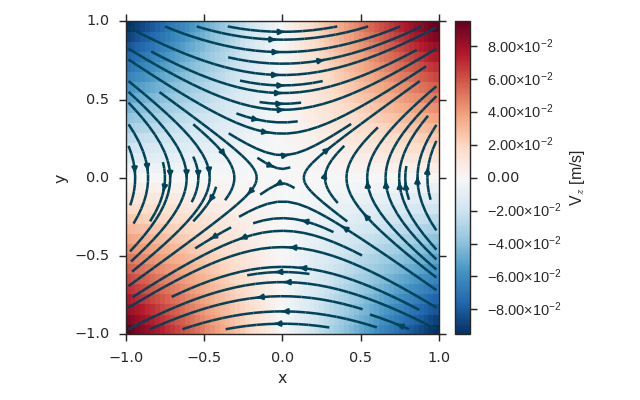
Vector Field
import numpy as np
import viscid
from viscid.plot import vpyplot as vlt
import matplotlib.pyplot as plt


x = np.linspace(-1, 1, 64)
y = np.linspace(-1, 1, 32)
z = np.linspace(-1, 1, 5)

fld = viscid.empty([x, y, z], nr_comps=3, layout='interlaced',
                   name="VFld1", pretty_name="Velocity [m/s]")
X, Y, Z = fld.get_crds(shaped=True)

# set the x, y, and z vector components separately
fld['x'] = 0.0 * X + 2.0 * Y + 0.0 * Z
fld['y'] = 1.0 * X + 0.0 * Y + 0.0 * Z
fld['z'] = 0.1 * (X * Y)

plt.figure(figsize=(8, 5))
vlt.plot(fld['z']['z=0j'], cbarlabel="V$_z$ [m/s]")
vlt.streamplot(fld['z=0j'])
vlt.auto_adjust_subplots()
plt.show()
(Source code, png)
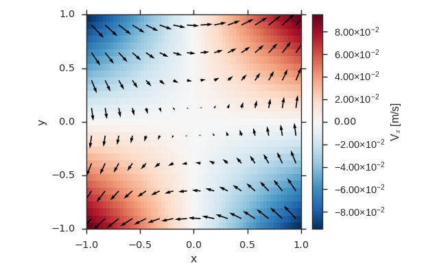
Vector Field on the Same Grid as a Scalar Field
import numpy as np
import viscid
from viscid.plot import vpyplot as vlt
import matplotlib.pyplot as plt


x = np.linspace(-1, 1, 64)
y = np.linspace(-1, 1, 32)

fld1 = viscid.empty([x, y], center='cell', name="ScalarFld",
                    pretty_name="Scalar Field")

# create fld2 using the same coordinates as fld1
fld2 = viscid.empty(fld1.crds, nr_comps=3, name="VectorFld",
                    pretty_name="Vector Field")

X, Y = fld2.get_crds(shaped=True)
fld2['x'] = 0.0 * X + 1.0 * Y
fld2['y'] = 1.0 * X + 0.0 * Y
fld2['z'] = 0.1 * (X * Y)

plt.figure(figsize=(8, 5))
vlt.plot(fld2['z'], cbarlabel="V$_z$ [m/s]")
vlt.plot2d_quiver(fld2, step=4)
vlt.auto_adjust_subplots()
plt.show()
(Source code, png)
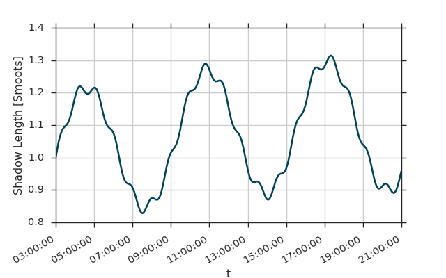
Datetime Time-Series
import matplotlib.dates as mdates
import numpy as np
import viscid
from viscid.plot import vpyplot as vlt
import matplotlib.pyplot as plt


t = viscid.linspace_datetime64('2010-06-23T03:00:00.0',
                               '2010-06-23T21:00:00.0', 256)

fld = viscid.empty([t], crd_names=['t'], center='node', name="TSeries",
                   pretty_name="Shadow Length [Smoots]")

t_sec = (fld.get_crd('t') - fld.get_crd('t')[0]) / np.timedelta64(1, 's')
fld[:] = (0.02 * np.sin(t_sec / (0.15 * 3600.0)) +
          0.20 * np.sin(t_sec / (1.0 * 3600.0)) +
          0.10 * np.sin(t_sec / (10.0 * 3600.0)) +
          1.0)

plt.figure(figsize=(8, 5))

vlt.plot(fld)

dateFmt = mdates.DateFormatter('%H:%M:%S')
plt.gca().xaxis.set_major_formatter(dateFmt)
plt.gcf().autofmt_xdate()
plt.gca().grid(True)

plt.show()
(Source code, png)
Wrapping Existing Ndarrays
You can also wrap pre-existing ndarrays directly,
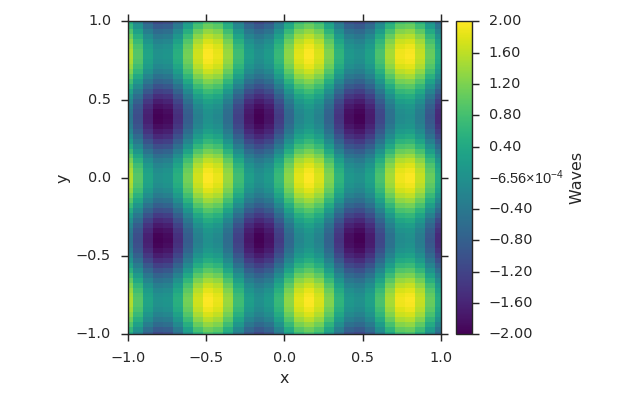
arrays2field
viscid.arrays2field() creates a field from existing ndarrays for coordinates and data.
import numpy as np
import viscid
from viscid.plot import vpyplot as vlt
import matplotlib.pyplot as plt


x = np.linspace(-1.0, 1.0, 32)
y = np.linspace(-1.0, 1.0, 64)
dat = np.sin(10 * x.reshape(-1, 1)) + np.cos(8 * y.reshape(1, -1))

fld = viscid.arrays2field([x, y], dat, name="Waves")
plt.figure(figsize=(8, 5))
vlt.plot(fld)
vlt.auto_adjust_subplots()
plt.show()
(Source code, png)
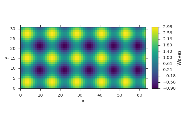
dat2field
viscid.dat2field() generates its own coordinates similar to matplotlib.pyplot.imshow(), i.e., using numpy.arange().
import numpy as np
import viscid
from viscid.plot import vpyplot as vlt
import matplotlib.pyplot as plt


x = np.linspace(-1.0, 1.0, 64).reshape(-1, 1)
y = np.linspace(-1.0, 1.0, 32).reshape(1, -1)
dat = 1.0 - np.sin(16 * x) + np.cos(8 * y)

fld = viscid.dat2field(dat, name="Waves")
plt.figure(figsize=(8, 5))
vlt.plot(fld)
vlt.auto_adjust_subplots()
plt.show()
(Source code, png)
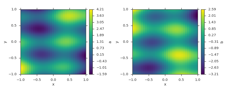
Wrapping Fields in Grids
Fields that are defined on the same grid at the same point in time can be added to a grid object. Do note however that this functionality is only intended to be used by readers. This is accentuated by the fact that the viscid.grid.Grid is not in the top-level namespace.
import numpy as np
import viscid
from viscid.plot import vpyplot as vlt
import matplotlib.pyplot as plt


grid = viscid.grid.Grid()

grid.crds = viscid.arrays2crds([np.linspace(-1, 1, 32),
                                np.linspace(-1, 1, 64)])
grid.add_field(viscid.full(grid.crds, np.nan, name='a'))
grid.add_field(viscid.full(grid.crds, np.nan, name='b'))

X, Y = grid.get_crds_cc(shaped=True)
grid['a'][...] = 1.0 + np.sin(4 * X) + np.cos(8 * Y) + 2.0 * X * Y
grid['b'][...] = np.sin(4 * X) - np.cos(8 * Y) - 2.0 * X * Y

_, (ax0, ax1) = plt.subplots(1, 2, figsize=(12, 5))
vlt.plot(grid['a'], ax=ax0)
vlt.plot(grid['b'], ax=ax1)
vlt.auto_adjust_subplots()
plt.show()
(Source code, png)