Magnetic Topology
Magnetic topology can be determined by the end points of magnetic field lines. By default, the topology output from calc_streamlines is a bitmask of closed (1), open-north (2), open-south (4), and solar wind (8). Any value larger than 8 indicates something else happened with that field line, such as reaching maxit or max_length and ending without hitting a boundary. The topology output can be switched to the raw boundary bitmask by giving topo_style='generic' as an argument to calc_streamlines.
For more info on streamlines, check out viscid.calc_streamlines() and subclasses of viscid.SeedGen
X-Point Location and Separator Tracing
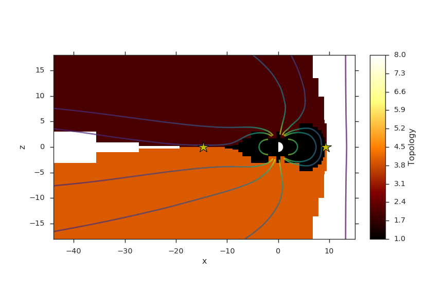
Bisection algorithm
This algorithm takes a 2d map in the uv space of a seed generator and iteratively bisects it into 4 quadrants. If the perimeter of a quadrant contains all 4 global topologies, the bisection continues in that quadrant. This has the advantage of uniquely finding all separator points to a given precision that is determined by the maximum number of iterations. This method is superior in most ways than the bit-or algorithm, but it is less extensively tested.
from os import path

import numpy as np
import viscid
from viscid.plot import vpyplot as vlt
from matplotlib import pyplot as plt


viscid.readers.openggcm.GGCMFile.read_log_file = True
viscid.readers.openggcm.GGCMGrid.mhd_to_gse_on_read = 'auto'


f3d = viscid.load_file(path.join(viscid.sample_dir, 'sample_xdmf.3d.xdmf'))
B = f3d['b']['x=-40j:15j, y=-20j:20j, z=-20j:20j']

# for this method, seeds must be a SeedGen subclass, not a field subset
seeds = viscid.Volume(xl=(-40, 0, -20), xh=(15, 0, 20), n=(64, 1, 128))

trace_opts = dict(ibound=2.5)
xpts = viscid.get_sep_pts_bisect(B, seeds, trace_opts=trace_opts)

# all done, now just make some illustration
log_bmag = np.log(viscid.magnitude(B))
lines, topo = viscid.calc_streamlines(B, seeds, **trace_opts)

vlt.plot(topo, cmap='afmhot')

vlt.plot2d_lines(lines[::79], scalars=log_bmag, symdir='y')
plt.plot(xpts[0], xpts[2], 'y*', ms=20,
             markeredgecolor='k', markeredgewidth=1.0)
plt.xlim(topo.xl[0], topo.xh[0])
plt.ylim(topo.xl[2], topo.xh[2])

# since seeds is a Field, we can use it to determine mhd|gse
vlt.plot_earth(B['y=0j'])

vlt.show()
(Source code, png)

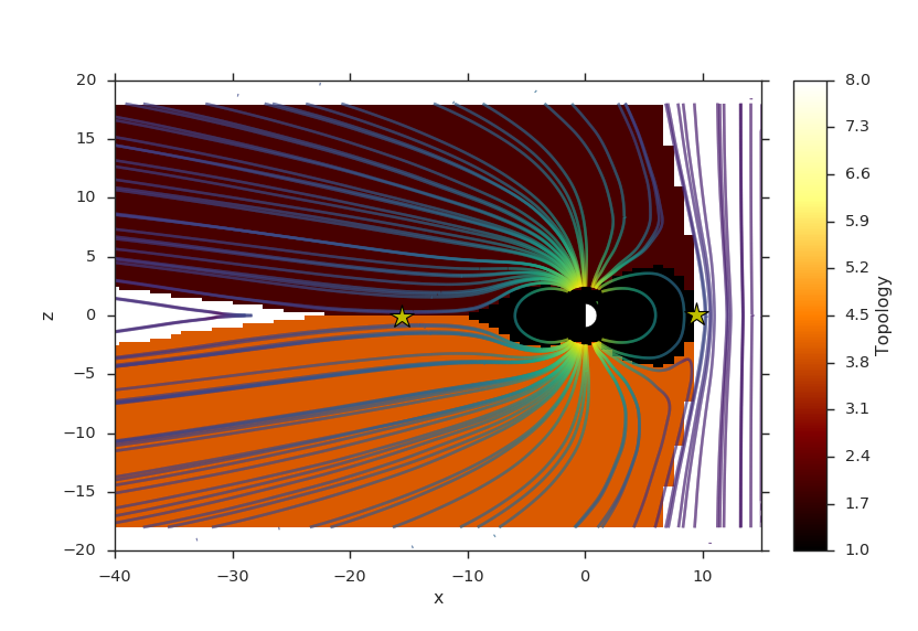
Bit-or algorithm
This algorithm takes a 2d map in the uv space of a seed generator and performs an iterative bitwise-or on neighbors until the intersection of all four global topologies meet. This algorithm is simple, but fragile. The more extended the reconnection region, the worse this algorithm will work. Also, do to the need for a clustering step, it is impossible to determine the accuracy of this method a priori.
from os import path

import numpy as np
import viscid
from viscid.plot import vpyplot as vlt
from matplotlib import pyplot as plt


viscid.readers.openggcm.GGCMFile.read_log_file = True
viscid.readers.openggcm.GGCMGrid.mhd_to_gse_on_read = 'auto'


f3d = viscid.load_file(path.join(viscid.sample_dir, 'sample_xdmf.3d.xdmf'))
B = f3d['b']['x=-40j:15j, y=-20j:20j, z=-20j:20j']

# for this method, seeds must be a SeedGen subclass, not a field subset
seeds = viscid.Volume(xl=(-40, 0, -20), xh=(15, 0, 20), n=(64, 1, 128))
seeds_dy = viscid.Volume(xl=(3, 0, -10), xh=(15, 0, 10), n=(64, 1, 128))
seeds_nt = viscid.Volume(xl=(-40, 0, -3), xh=(-5, 0, 3), n=(64, 1, 128))

trace_opts = dict(ibound=2.5)
xpts_dy = viscid.get_sep_pts_bitor(B, seeds_dy, trace_opts=trace_opts)
xpts_nt = viscid.get_sep_pts_bitor(B, seeds_nt, trace_opts=trace_opts)

# all done, now just make some illustration
log_bmag = np.log(viscid.magnitude(B))
lines, topo = viscid.calc_streamlines(B, seeds, **trace_opts)
_, topo_dy = viscid.calc_streamlines(B, seeds_dy, ibound=3.0,
                                     output=viscid.OUTPUT_TOPOLOGY)
_, topo_nt = viscid.calc_streamlines(B, seeds_nt, ibound=3.0,
                                     output=viscid.OUTPUT_TOPOLOGY)

clim = (np.min(topo), np.max(topo))
vlt.plot(topo, cmap='afmhot', clim=clim)
vlt.plot(topo_dy, cmap='afmhot', clim=clim, colorbar=None)
vlt.plot(topo_nt, cmap='afmhot', clim=clim, colorbar=None)

vlt.plot2d_lines(lines[::79], scalars=log_bmag, symdir='y')
plt.plot(xpts_dy[0], xpts_dy[2], 'y*', ms=20,
             markeredgecolor='k', markeredgewidth=1.0)
plt.plot(xpts_nt[0], xpts_nt[2], 'y*', ms=20,
             markeredgecolor='k', markeredgewidth=1.0)
plt.xlim(topo.xl[0], topo.xh[0])
plt.ylim(topo.xl[2], topo.xh[2])

# since seeds is a Field, we can use it to determine mhd|gse
vlt.plot_earth(B['y=0j'])

vlt.show()
(Source code, png)

The bit-or algorithm can has another interface that just takes a topology field. It can be used this way:
from os import path

import numpy as np
import viscid
from viscid.plot import vpyplot as vlt
from matplotlib import pyplot as plt


viscid.readers.openggcm.GGCMFile.read_log_file = True
viscid.readers.openggcm.GGCMGrid.mhd_to_gse_on_read = 'auto'


f3d = viscid.load_file(path.join(viscid.sample_dir, 'sample_xdmf.3d.xdmf'))
B = f3d['b']['x=-40j:15j, y=-20j:20j, z=-20j:20j']

# Fields can be used as seeds to get one seed per grid point
seeds = B.slice_keep('y=0j')
lines, topo = viscid.calc_streamlines(B, seeds, ibound=2.5,
                                      output=viscid.OUTPUT_BOTH)
xpts_night = viscid.topology_bitor_clusters(topo['x=:0j, y=0j'])

# The dayside is done separately here because the sample data is at such
# low resolution. Super-sampling the grid with the seeds can sometimes help
# in these cases.
day_seeds = viscid.Volume((7.0, 0.0, -5.0), (12.0, 0.0, 5.0), (16, 1, 16))
_, day_topo = viscid.calc_streamlines(B, day_seeds, ibound=2.5,
                                      output=viscid.OUTPUT_TOPOLOGY)
xpts_day = viscid.topology_bitor_clusters(day_topo)

log_bmag = np.log(viscid.magnitude(B))

clim = (min(np.min(day_topo), np.min(topo)),
        max(np.max(day_topo), np.max(topo)))
vlt.plot(topo, cmap='afmhot', clim=clim)
vlt.plot(day_topo, cmap='afmhot', clim=clim, colorbar=None)

vlt.plot2d_lines(lines[::79], scalars=log_bmag, symdir='y')
plt.plot(xpts_night[0], xpts_night[1], 'y*', ms=20,
             markeredgecolor='k', markeredgewidth=1.0)
plt.plot(xpts_day[0], xpts_day[1], 'y*', ms=20,
             markeredgecolor='k', markeredgewidth=1.0)
plt.xlim(topo.xl[0], topo.xh[0])
plt.ylim(topo.xl[2], topo.xh[2])

# since seeds is a Field, we can use it to determine mhd|gse
vlt.plot_earth(seeds.slice_reduce(":"))

vlt.show()
(Source code, png)