Slicing Fields
The syntax and semantics for indexing are almost equivalent to Numpy’s basic indexing. The key difference is Viscid supports slice-by-location (complex numbers, see below). Also, Viscid supports indexing by arrays (like Numpy’s advanced indexing), but these arrays must be one-dimensional. Unfortunately, true advanced indexing is poorly defined when the result has to be on a grid.
See Indexing Fields for a complete enumeration of slicing rules.
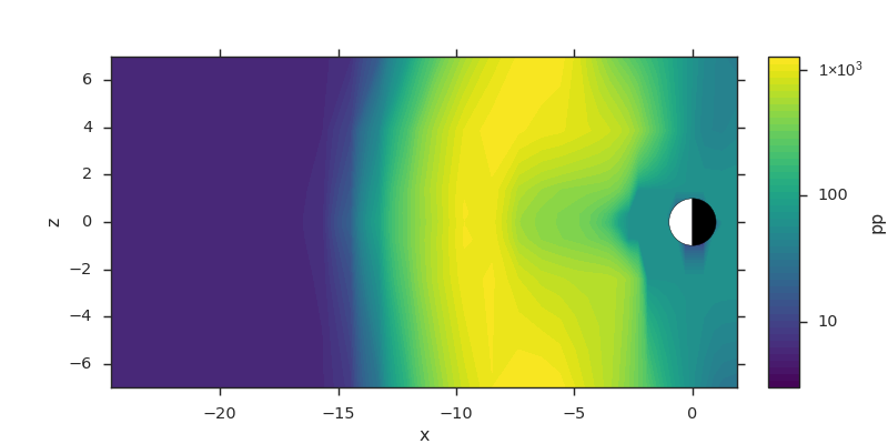
Spatial Slices
The following example shows how to slice the x axis by index, and the {y, z} axes by location. Note that slices can be given as strings to be explicit about which axes you want sliced.
from os import path

import viscid
from viscid.plot import vpyplot as vlt
from matplotlib import pyplot as plt


f3d = viscid.load_file(path.join(viscid.sample_dir, 'sample_xdmf.3d.xdmf'))

# snip off the first 5 and last 25 cells in x, and grab every other cell
# in z between z = -8.0 and z = 10.0 (in space, not index).
# Notice that slices by location are done by appending an 'j' to the
# slice. This means "y=0" is not the same as "y=0j".

pp = f3d["pp"][5:-25, 0.0j, -8.0j:10.0j:2]

# this slice is also equivalent to...
# >>> pp = f3d["pp"]["x = 5:-25", "y = 0.0j", "z = -8.0j:10.0j:2"]
# >>> pp = f3d["pp"]["x = 5:-25, y = 0.0j, z = -8.0j:10.0j:2"]

plt.subplots(1, 1, figsize=(10, 5))
vlt.plot(pp, style="contourf", levels=50, plot_opts="log,earth")

vlt.show()
(Source code, png)

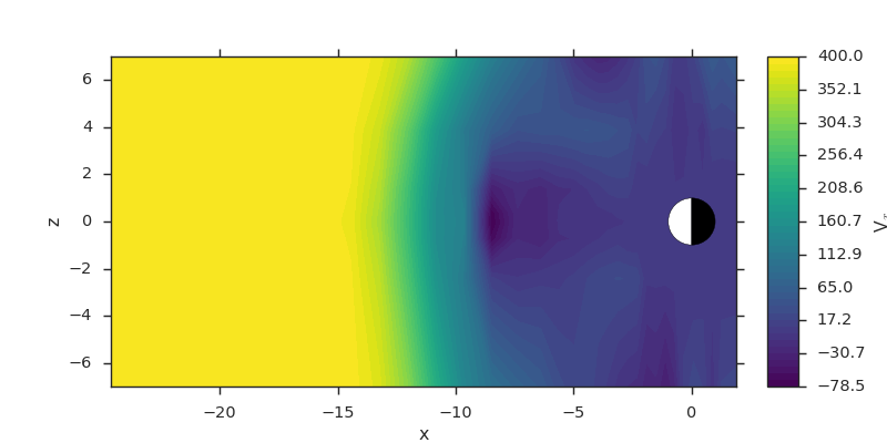
Vector Component Slices
Slices of vector fields are spatial slices that are invariant of the data layout. Single components can be extracted by the component name (usually one of “xyz”).
from os import path

import viscid
from viscid.plot import vpyplot as vlt
from matplotlib import pyplot as plt


f3d = viscid.load_file(path.join(viscid.sample_dir, 'sample_xdmf.3d.xdmf'))

vx = f3d["v"]["x, x = 5:-25, y = 0.0j, z = -8.0j:10.0j:2"]

# this slice is also equivalent to...
# >>> vx = f3d["vx"]["x = 5:-25", "y = 0.0j", "z = -8.0j:10.0j:2"]

plt.subplots(1, 1, figsize=(10, 5))
vlt.plot(vx, style="contourf", levels=50, plot_opts="earth")

vlt.show()
(Source code, png)
Temporal Slices
Temporal Datasets can be sliced a number of ways too, here are some examples
>>> from os import path
>>>
>>> import viscid
>>>
>>>
>>> f3d = viscid.load_file(path.join(viscid.sample_dir, 'sample_xdmf.3d.xdmf'))
>>>
>>> grids = f3d.get_times(slice("UT1967:01:01:00:10:00.0",
>>>                             "UT1967:01:01:00:20:00.0"))
>>> print([grid.time for grid in grids])
[600.0, 1200.0]
>>>
>>> grids = f3d.get_times(1)
>>> print([grid.time for grid in grids])
[600.0]
>>>
>>> grids = f3d.get_times(slice(None, 600.0))
>>> print([grid.time for grid in grids])
[600.0]
>>> grids = f3d.get_times("T0:10:00.0:T0:20:00.0")
>>> print([grid.time for grid in grids])
[600.0, 1200.0]
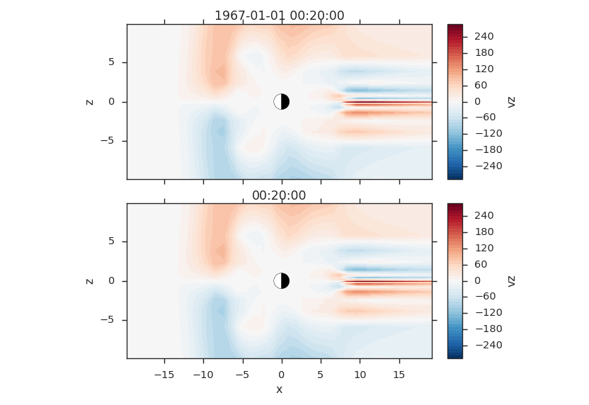
Single Time Slice
from os import path

import viscid
from viscid.plot import vpyplot as vlt
from matplotlib import pyplot as plt


f3d = viscid.load_file(path.join(viscid.sample_dir, 'sample_xdmf.3d.xdmf'))

_, axes = plt.subplots(2, 1, sharex=True, sharey=True)
f3d.activate_time(0)

# notice y=0.0, this is different from y=0; y=0 is the 0th index in
# y, which is this case will be y=-50.0
vlt.plot(f3d["vz"]["x = -20.0j:20.0j, y = 0.0j, z = -10.0j:10.0j"],
         style="contourf", levels=50, plot_opts="lin_0,earth", ax=axes[0])
plt.title(f3d.get_grid().format_time("UT"))

# share axes so this plot pans/zooms with the first
f3d.activate_time(-1)
vlt.plot(f3d["vz"]["x = -20.0j:20.0j, y = 0.0j, z = -10.0j:10.0j"],
         style="contourf", levels=50, plot_opts="lin_0,earth", ax=axes[1])
plt.title(f3d.get_grid().format_time("hms"))

vlt.auto_adjust_subplots()
vlt.show()
(Source code, png)

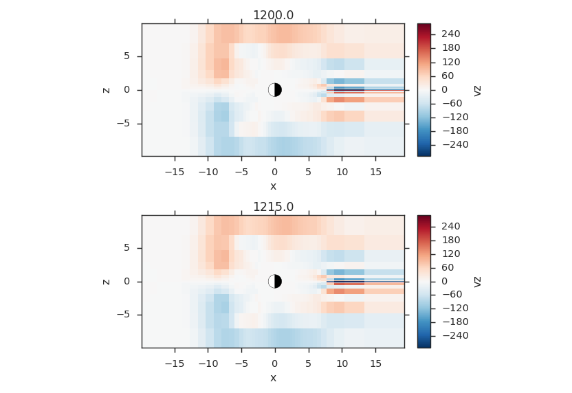
Iterating Over Time Slices
Or, if you need to iterate over all time slices, you can do that too. The advantage of using the iterator here is that it’s smart enough to kick the old time slice out of memory when you move to the next time.
from os import path

import numpy as np
import viscid
from viscid.plot import vpyplot as vlt
from matplotlib import pyplot as plt


f2d = viscid.load_file(path.join(viscid.sample_dir, 'sample_xdmf.py_0.xdmf'))

times = np.array([grid.time for grid in f2d.iter_times(":2")])
nr_times = len(times)

_, axes = plt.subplots(nr_times, 1)

for i, grid in enumerate(f2d.iter_times(":2")):
    vlt.plot(grid["vz"]["x = -20.0j:20.0j, y = 0.0j, z = -10.0j:10.0j"],
             plot_opts="lin_0,earth", ax=axes[i])
    plt.title(grid.format_time(".01f"))

vlt.auto_adjust_subplots()
vlt.show()
(Source code, png)