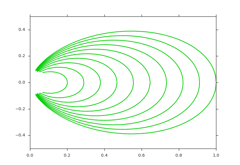
Streamlines
Streamlines require a VectorField and a seed generator. If you just want a single streamline, you can also use an (x, y, z) tuple. For a more comprehensive list of seed generators, check out Useful Functions or to see them in action, run Viscid/tests/test_seed.py.
A more in-depth example of using and plotting streamlines can be found in the Quasi Potential Example.
import numpy as np
import viscid
from viscid.plot import vpyplot as vlt
from matplotlib import pyplot as plt


B = viscid.make_dipole(twod=True)
obound0 = np.array([-4, -4, -4], dtype=B.data.dtype)
obound1 = np.array([4, 4, 4], dtype=B.data.dtype)
lines, topo = viscid.calc_streamlines(B,
                                      viscid.Line((0.2, 0.0, 0.0),
                                                  (1.0, 0.0, 0.0), 10),
                                      ds0=0.01, ibound=0.1, maxit=10000,
                                      obound0=obound0, obound1=obound1,
                                      method=viscid.EULER1,
                                      stream_dir=viscid.DIR_BOTH,
                                      output=viscid.OUTPUT_BOTH)
topo_colors = viscid.topology2color(topo)
vlt.plot2d_lines(lines, topo_colors, symdir='y')
plt.ylim(-0.5, 0.5)

vlt.show()
(Source code, png)

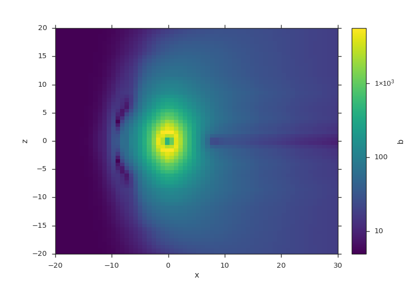
Interpolation
Interpolating Onto a Volume
from os import path

import viscid
from viscid.plot import vpyplot as vlt


f3d = viscid.load_file(path.join(viscid.sample_dir, 'sample_xdmf.3d.xdmf'))

seeds = viscid.Volume((-20, 1, -20), (30, 1, 20), n=(64, 5, 64))
b = viscid.interp_trilin(f3d['b'], seeds)
vlt.plot(viscid.magnitude(b)['y=0j'], logscale=True, earth=True)

vlt.show()
(Source code, png)

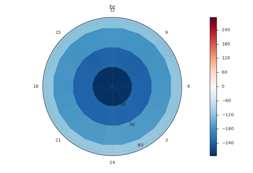
Interpolating Onto a Sphere
By default, spheres ore plotted in 2D via their phi (x-axis) and theta (y-axis).
from os import path

import viscid
from viscid.plot import vpyplot as vlt


f3d = viscid.load_file(path.join(viscid.sample_dir, 'sample_xdmf.3d.xdmf'))

b = viscid.interp_trilin(f3d['bz'], viscid.Sphere(p0=(0, 0, 0), r=7.0))
vlt.plot(b, lin=0, hemisphere='north')

vlt.show()
(Source code, png)

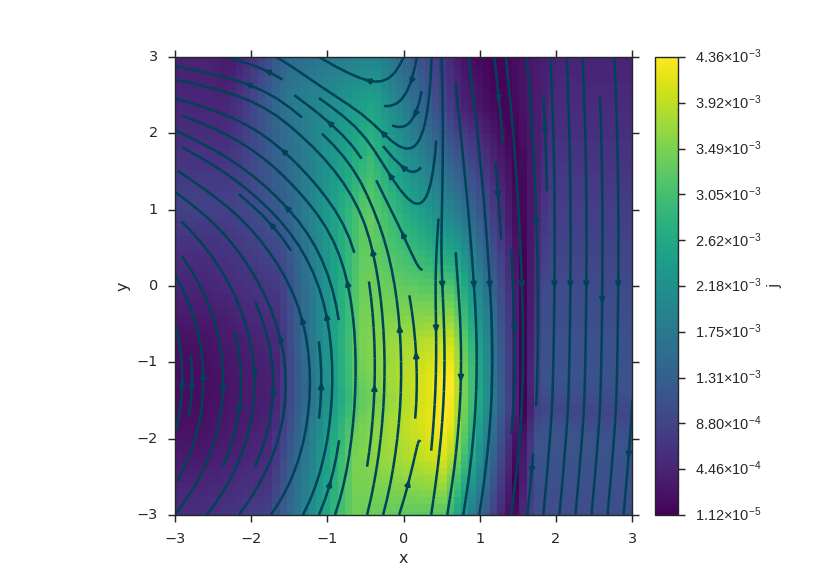
Interpolating Vectors Onto a Plane
from os import path

import numpy as np
import viscid
from viscid.plot import vpyplot as vlt


viscid.readers.openggcm.GGCMFile.read_log_file = True
viscid.readers.openggcm.GGCMGrid.mhd_to_gse_on_read = 'auto'


f3d = viscid.load_file(path.join(viscid.sample_dir, 'sample_xdmf.3d.xdmf'))

# make N and L directions for LMN magnetopause boundary normal crds
p0 = (9.0, 0.0, 1.5)
plane = viscid.Plane(p0, pN=[0, -1, 0], pL=[1, 0, 0.05], len_l=[-3, 3],
                     len_m=6.0, nl=64, nm=64)
slc = "x=6j:11j, y=-1j:1j, z=-10j:10j"
b = viscid.interp_trilin(f3d['b'][slc], plane)
j = viscid.interp_trilin(f3d['j'][slc], plane)

# rotate the vector so its components are in / normal to the plane
# that we interpolated onto
xyz_to_lmn = plane.get_rotation().T
b = b.wrap(np.einsum("ij,lm...j->lm...i", xyz_to_lmn, b))
j = j.wrap(np.einsum("ij,lm...j->lm...i", xyz_to_lmn, j))

vlt.plot(viscid.magnitude(j))
vlt.streamplot(b)

vlt.show()
(Source code, png)