Plotting Vector Quantities

Various shims for plotting fields using matplotlib are provided by viscid.plot.vpyplot. The functions are listed in Useful Functions. For an enumeration of extra plotting keyword arguments, see Plot Options. Also, you can specify keyword arguments that are conusmed by the matplotlib function used to make the plot, i.e., pyplot.streamline, pyplot.quiver, etc.

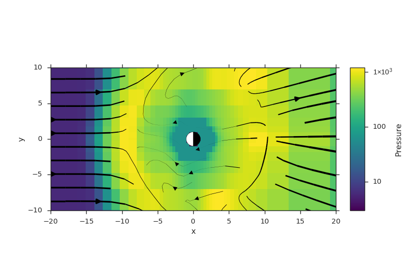
Streamplot

Plotting 2D streamlines. Note that using matplotlib to make streamlines from a 2D slice may make it appear that Div B ≠ 0, but that’s just an illusion. If this is a problem, you can always resort to full 3D streamlines, as in Streamlines.

from os import path

import viscid
from viscid.plot import vpyplot as vlt
from matplotlib import pyplot as plt


viscid.calculator.evaluator.enabled = True


f3d = viscid.load_file(path.join(viscid.sample_dir, 'sample_xdmf.3d.xdmf'))

vlt.plot(f3d['Pressure = pp']['z=0j'], logscale=True, earth=True)

v = f3d['v']
speed = viscid.magnitude(v)
lw = 4 * speed / speed.max()
slc = 'z=0j'
vlt.streamplot(v[slc], arrowsize=2, density=2, linewidth=lw[slc], color='k')

plt.xlim(-20, 20)
plt.ylim(-10, 10)

vlt.show()

(Source code, png)

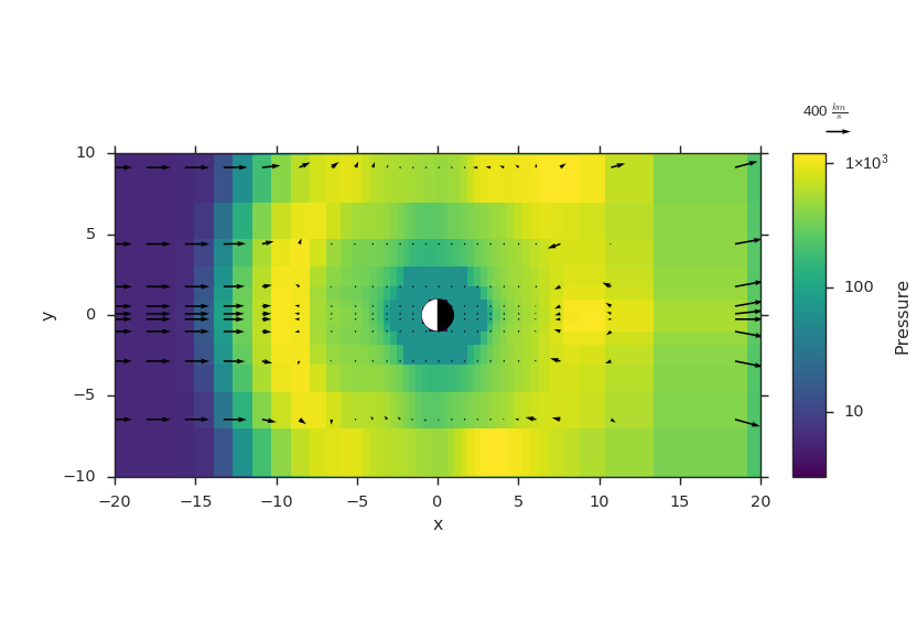
Quivers

Quivers are another way to show vector fields, but in many cases, it will be useful to downsample the field, or else there will be far too many arrows.

from os import path

import viscid
from viscid.plot import vpyplot as vlt
from matplotlib import pyplot as plt


f3d = viscid.load_file(path.join(viscid.sample_dir, 'sample_xdmf.3d.xdmf'))

vlt.plot(f3d['pp']['z=0j'], cbarlabel="Pressure", logscale=True, earth=True)
Q = vlt.plot2d_quiver(f3d['v']['x=::2, y=::2, z=0j'])
plt.quiverkey(Q, X=1.1, Y=1.07, U=400, label=r"400 $\frac{km}{s}$",
              labelpos='N')

plt.xlim(-20, 20)
plt.ylim(-10, 10)

vlt.show()

(Source code, png)

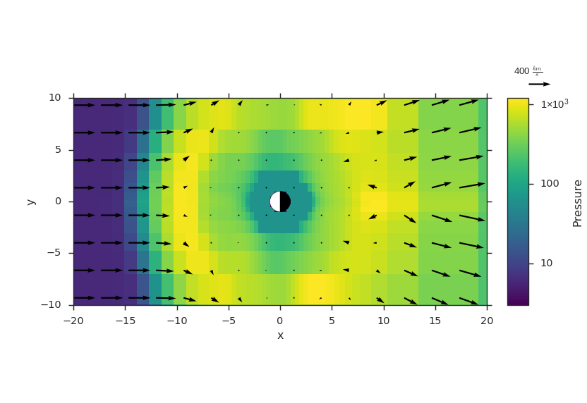
Uniform Quivers

If your data has a very nonuniform grid, it may be useful to interpolate your data onto a uniform grid first.

from os import path

import viscid
from viscid.plot import vpyplot as vlt
from matplotlib import pyplot as plt


viscid.calculator.evaluator.enabled = True


f3d = viscid.load_file(path.join(viscid.sample_dir, 'sample_xdmf.3d.xdmf'))

vlt.plot(f3d['Pressure = pp']['z=0j'], logscale=True, earth=True)
new_grid = viscid.Volume((-20, -20, 0), (20, 20, 0), n=(16, 16, 1))
v = viscid.interp_trilin(f3d['v'], new_grid)
Q = vlt.plot2d_quiver(v['z=0j'])
plt.quiverkey(Q, X=1.1, Y=1.07, U=400, label=r"400 $\frac{km}{s}$",
              labelpos='N')


plt.xlim(-20, 20)
plt.ylim(-10, 10)

vlt.show()

(Source code, png)